Computational model calibration

Calibration, or parameter estimation, consists in solving the inverse problem of finding descriptors (species, parameters or compartments) values such that the computational model outputs match some user-defined fitness criteria.

Fitness function

The fitness is a metric of the match between outputs of the simulation and the expected behaviors that are covered by the Objectives in the Advanced oupt sets and / or the data tables used as calibration inputs. 

The 'Outputs' tab of the calibration consists of a list of output sets and / or data tables, where having at least one item selected is mandatory. The fitness function will be defined as the weigthed sum of the different elements defined as objectives in the Advanced output set and the data tables. In the calibration results, it it called 'optimizationWeigthedScore'.Other outputs(scalar or time series) can also be used in a calibration, but they will only be output for visualization and not used in the fitness function.

Output sets

In Jinkō, you can create two types of output sets

• Simple output sets allow to define the time series and scalar outputs to be visualized as output of a trial.
• Advanced output sets also allow to define some scalar outputs but with more flexibility by using formulas, and more importantly in the context of a calibration, it allows to define objectives and constraints that will be used in the the fitness function. As opposed to the data tables, these objectives and constraints can be qualitative and not directly data.

The output sets are further detailed in the specific documentation, when you can learn how to define outputs.

Data table

Format

To be used in a calibration, a data-table must have its columns abide by the following format, here described in the form of a JSON schema:

{
  "oneOf": [
    {
      "properties": {
        "obsId": {
          "type": "string"
        },
        "time": {
          "type": "string",
          "format": "ISO8601"
        },
        "value": {
          "type": "number"
        },
        "unit": {
          "type": "string",
          "format": "physical_unit"
        },
        "armScope": {
          "type": "string"
        },
        "wideRangeLowBound": {
          "type": "number"
        },
        "wideRangeHighBound": {
          "type": "number"
        },
        "weight": {
          "type": "number",
          "minimum": 0
        },
        "experimentRef": {
          "type": "string"
        }
      },
      "required": [
        "obsId",
        "time",
        "value"
      ],
      "type": "object"
    },
    {
      "properties": {
        "obsId": {
          "type": "string"
        },
        "time": {
          "type": "string",
          "format": "ISO8601"
        },
        "narrowRangeLowBound": {
          "type": "number"
        },
        "narrowRangeHighBound": {
          "type": "number"
        },
        "unit": {
          "type": "string",
          "format": "physical_unit"
        },
        "armScope": {
          "type": "string"
        },
        "wideRangeLowBound": {
          "type": "number"
        },
        "wideRangeHighBound": {
          "type": "number"
        },
        "weight": {
          "type": "number",
          "minimum": 0
        },
        "experimentRef": {
          "type": "string"
        }
      },
      "required": [
        "obsId",
        "time",
        "narrowRangeLowBound",
        "narrowRangeHighBound"
      ],
      "type": "object"
    }
  ]
}

More details about the format

· obsId (required)

An advanced output formula describing the quantity of interest derived from the computational model to be compared with the data. In particular, it may be a simple reference to a model constituent, i.e. the identifier of a parameter, compartment or species.

· time (required)

Time of the observation following the ISO 8601 duration format.

💡 In Jinkō's web interface, you may also have plain numbers in this column provided that the time unit is specified in the CSV header with time(<time_unit>) where <time_unit> can be any of second, minute, hour, day, week, month and year. We are currently working on supporting this feature when using the API as well.

· value (required if narrowRangeLowBound and narrowRangeHighBound are unset)

A real number representing the observed value of obsId at time time. The calibration score is equal to $1$ if the simulated value is equal to value and decreases towards $-\infty$ as it gets further away from it. The following table of variation summarizes the behavior of the score as a function of obsId:

$$\begin{array}{|c|ccccccccr|} \hline \mathrm{obsId} & -\infty & & \mathrm{wideRangeLowBound} & & \mathrm{value} & & \mathrm{wideRangeHighBound} & & +\infty \\ \hline & & & & & 1 & & & & +\infty \\ & & & & \nearrow & & \searrow & & & \\ \mathrm{score} & & & 0 & & & & 0 & & \\ & & \nearrow & & & & & & \searrow & \\ & -\infty & & & & & & & & -\infty \\ \hline \end{array}$$

· narrowRangeLowBound and narrowRangeHighBound (required if value is unset)

Two real values describing the "narrow range" of values taken by obsId within which the score is equal to $1$. In this case, the table of variations becomes:

$$\begin{array}{|c|ccccccccccr|} \hline \mathrm{obsId} & -\infty & & \mathrm{wideRangeLowBound} & & \mathrm{narrowRangeLowBound} & & \mathrm{narrowRangeHighBound} & & \mathrm{wideRangeHighBound} & & +\infty \\ \hline & & & & & 1 & & 1 & & & & \\ & & & & \nearrow & & & & \searrow & & & \\ \mathrm{score} & & & 0 & & & & & & 0 & & \\ & & \nearrow & & & & & & & & \searrow & \\ & -\infty & & & & & & & & & & -\infty \\ \hline \end{array}$$

💡 Setting both value and (narrowRangeLowBound,narrowRangeHighBound) is redundant but not considered an error. In case both are set, (narrowRangeLowBound,narrowRangeHighBound) takes precedence and value is discarded.

· wideRangeLowBound and wideRangeHighBound (optional)

Two real values describing a "wide range". When obsId is between the "wide range" and the "narrow range", the score varies continuously from 0 to 1 (see the above tables of variations).

When unset, the wide range defaults to $(\mathrm{narrowRangeLowBound} - 1, \mathrm{narrowRangeHighBound} + 1)$. In such a case, the resulting objective function becomes equivalent to a mean squared error $f(x) = 1 - (x- x^*)^2$ where $x^*$ is either narrowRangeLowBound (resp. narrowRangeRightBound) when $x \le \mathrm{narrowRangeLowBound}$ (resp. $x \ge \mathrm{narrowRangeHighBound}$) or just value.

The following figure shows an example of the score as a function of $x$ (the simulated value of obsId at a given time) where

• wideRangeLowBound = 3
• narrowRangeLowBound = 5
• narrowRangeHighBound = 6
• wideRangeHighBound = 7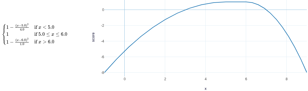

· armScope (optional)

Specifies in which protocol arm the data table row applies. Must obey the following consistency rules with respect to obsId:

• If obsId references a single protocol arm then armScope, if set, must be equal to that arm
• If obsId references two or more arms, armScope must be unset
• If obsId does not reference any protocol arm, then armScope may be either set (row will apply to that arm only) or unset (row will apply to all arms). ⚠️ This is not considered good practice for it is ambiguous and can yield surprising results, notably regarding the relative weights. If your trial or calibration has two or more protocol arms, this will raise a warning.

· weight (optional)

Weight of the observation row. It will be used to compute a weighted mean for the score tied to each (obsId, armScope) pair. Defaults to 1.

· unit (optional)

The unit of the obsId values and narrow/wide ranges. This will be used to raise a warning in case the unit is different between the data table and the computational model, but it will not automatically convert the data. 

· experimentRef (optional)

A link to track where the data comes from, akin to the "links" fields of a computational model. 

Examples

Here is an example of a data-table in CSV format that may be used for calibration purposes: 

obsId,time,value,unit,armScope
AdcConcentration,P0D,0,ug/mL,control
AdcConcentration,P2D,11.1,ug/mL,control
AdcConcentration,P16D,7.56,ug/mL,control
AdcConcentration,P0D,0,ug/mL,treated_single_dose
AdcConcentration,P2D,9.64,ug/mL,treated_single_dose
AdcConcentration,P16D,5.16,ug/mL,treated_single_dose

Another example where we define "narrow ranges" instead of value:

obsId,time,narrowRangeLowBound,narrowRangeHighBound,unit,armScope,wideRangeLowBound,wideRangeHighBound,weight,experimentRef
AdcConcentration,PT0H,0,0,ug/mL,control,0,10,1,https://jinko.ai
AdcConcentration,PT16H,10.5,11.5,ug/mL,control,5,15,1,https://jinko.ai
AdcConcentration,PT150H,7,8,ug/mL,control,5,15,1,https://jinko.ai
AdcConcentration,PT0H,0,0,ug/mL,treated_single_dose,0,10,1,https://jinko.ai
AdcConcentration,PT150H,9,10,ug/mL,treated_single_dose,5,15,1,https://jinko.ai
AdcConcentration,PT250H,5,5.5,ug/mL,treated_single_dose,5,15,1,https://jinko.ai

Validation in Jinkō

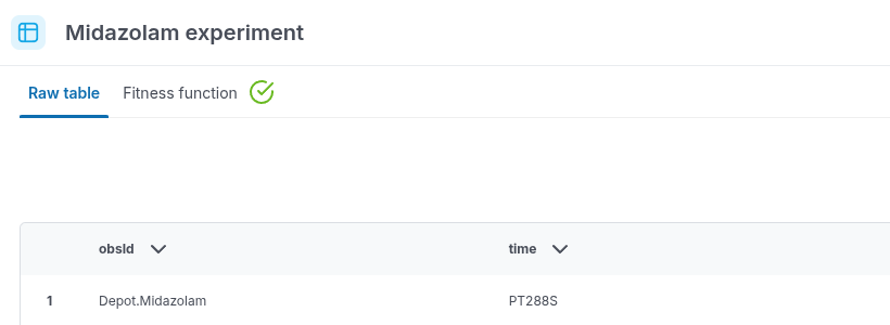
If the data-table you uploaded to https://jinko.ai conforms with the aforementioned fitness function schema, you will see a green tick next to the "Fitness function" tab:

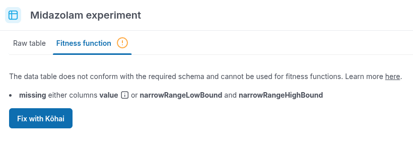
Otherwise, you will see the following warning sign along with a set of instructions to modify the data-table:

Algorithm

The calibration fitness function is defined as the weighted sum of the different fitness criteria. It produces a single scalar value, ranging from -∞ to 1, which the calibration algorithm aims at maximizing.

Under the hood, Jinkō uses the Covariance Matrix Adaptation Evolution Strategy (CMA-ES) algorithm to perform such maximization.

Running a calibration

Computational model, Output set and Protocol arms

To start off, you’ll need a computational model to calibrate. This model will be used to run the simulations with varying inputs (cf next section). 

You can also add an Output Set, if there are outputs of the model you’d like to observe. Note that unlike the scorings, which may also be output as scalar results, the output set will not be used for the optimization, but only for visualization. 

You can also add Protocol arms, in order to run your model in several different circumstances (typically, different types of experiments, or different doses of a trial).

Inputs to calibrate

The inputs to calibrate are the model components that will be used for the optimization of the weighted score. You will need to select here the parameters, species or compartments for which the values (respectively initial condition or volume) are unknown. You also need to ensure that the selected inputs actually have an impact on the outpurs you want to optimize: you can use the contribution analysis tool for that. 

For each selected input, you need to define:

• The mean and SD: the default values are taken from your CM, and will be used to define a normal distribution from which the patients for the first iteration will be drawn.

• The bounds are used in the calibration to penalize unacceptable values of a given parameter, typically to avoid wrong behaviors of the model, such as a KM parameter becoming negative. 

• For parameters that you need to explore on a large range, you can use a log transformation. In that case, In that case we perform a change of variables and calibrate the log of the parameter. This means in particular that the the mean and SD values are those of the log (i.e. you should put a mean of 1 if you want your parameter to be sampled around 10). 

Adding too many inputs to calibrate or very wide ranges will lead to the parameter space to explore being huge, and therefore maybe not fully explored. On the other hand, having a too small parameter space may not allow you to optimize your weighted score. It is usually recommended to have 3 to 10 inputs to calibrate, possibly by doing several iterative calibration steps.

Calibration and solving options

The calibration options are the options with which the algorithm will be run:

• Number of iterations (optional) is the maximum number of iterations that the calibration will run for. After this, the calibration will stop even if it has not reached a convergence. Filling this is optional: if it is not filled, it does not mean that the calibration will run infinitely, but rather that Jinkō will compute a number based on the number inputs to calibrate and the population size (default_number_of_iterations = 10 * (n+1)^2 / ( sqrt (default_pop_size)) where n is the number of inputs to calibrate).
• Population size (optional) is the number of patients to be drawn at each iteration. The larger the population size, the more the parameter space is explored at each iteration. Filling this is optional: if it is not filled, Jinkō will compute a number based on the number inputs to calibrate (default_pop_size = 4 + floor (3 * log (n)) where n is the number of inputs to calibrate).
• Seed (mandatory, defaults to 0) is an arbitrary integer that is used to initialize the random number generation. It is useful for reproducibility, or to add variability in the calibration: changing just this seed with all the same inputs will change the initialization of the calibration and therefore the results.
• Threshold weighted score (mandatory, defaults to 1) is the threshold used to determine the calibration success: the calibration stops as soon as one patient reaches this threshold.
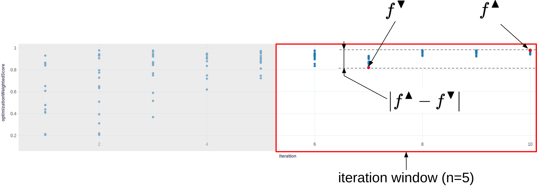
• The following options pertain to fitness function stagnation detection, turned on by default. When turned on, it will make the calibration stop earlier if there is no noticeable improvement in the fitness function over a certain number of iterations. The stopping criterion is defined as such: After a "burn-in" period, at each iteration, consider a set of the highest (i.e. the best) fitness function values for each of the last n iterations, let us call this set the "iteration window" and n the "iteration window size". Let us denote by f▲ (resp. f▼) the highest or "best" (resp. the lowest or "worst") value in the "iteration window". The fitness function is considered to be stagnating if the following condition is met:

Stagnation detection can be configured using the following four options:

• Stagnation burn in period (optional, defaults to 100) is the "burn-in" period after which stagnation detection is allowed to start
• Stagnation iteration window size (optional, defaults to 25) is the number of iterations comprised in the stagnation detection window
• Stagnation absolute tolerance (optional, defaults to 1e-3) is tol_abs in the above formula
• Stagnation relative tolerance (optional, defaults to 1e-3) is tol_rel in the above formula

The solving options are the options that will be used to solve each task. They are the same as for a trial simulation, and the most important one to check is probably the duration of a simulation.

Results and interpretation

Once your calibration has started running, a new section "Results" will appear in your calibration. As soon as the fiist iteration is finished, you will start to see the first results. You can also stop the calibration if you see that it is going in a wrong direction.

Here, you can see in the Summary tab:

• The progress across iterations, with a scatter plot and a table of the evolution across iterations. By default, this applies on the optimizationWeightedScore (i.e. the fitness function) but you can select any other descriptor to check its evolution and the Maximum and average for each iteration. In the table, you also have information on the iteration itself, such as the termination time, allowing to assess how much time each iteration lasts, the number of failed tasks (i.e. numerical resolution errors, one task being one model run, so one patient on one parameter arm) and out of bounds patients (patients for whom the algorithm drew values outside of the bounds defined in the inputs to calibrate). A lot of out of bound patients may mean that the bounds defined for the parameter space are too restrictive, and a lot of failed tasks may mean that the model is quite unstable, at least in this part of the parameter space.
• A scalar X-Y scatter plot, in which you can select input descriptors or outputs, in order to check the co-evolution of some scalars from the calibration. This can typically allow to check if there is a correlation between an input parameter and an objective, or a (negative) correlation between two objectives.

The Individual patients tab also allows to see the dynamics of individual patients, as in the trial. The patients are ranked by optimizationWeightedScore, starting with the best patient. If there are data tables defined as outputs, the data will be overlaid to the model outputs. In the app panel, you can see this specific patients inputs and outputs and export them as csv to reuse manually into the model, or you can use the "Update computational model" button to directly update the values of the calibrated inputs. This will also create a new version of the CM and add links to the calibration and it's version in the computational model (in the "links" field of these descriptors).

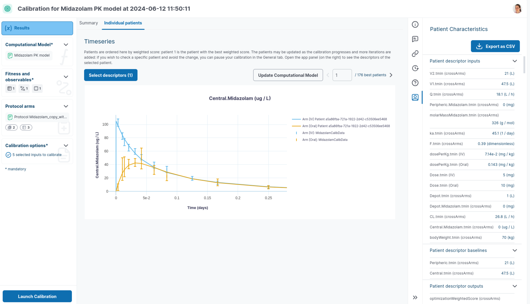
The calibration will stop either once one patient has reached the threshold defined in the calibration options, or once the maximum number of iterations has been reached. If you find a patient that you consider good enough before that, you can also stop the calibration to save computing power.

What if my calibration does not work?

There are a lot of reasons for a calibration to not work as expected. Whatever the changes needed are, you can edit all of the inputs directly in the calibration to correct them, and relaunch a new calibration run on a new version, unless you are re-using an existing project item, in which case you will be in read only mode. However, it is easy to make a copy of this PI and then edit it.

If a constraint is not respected, the patient will be penalized and the optimizationWeightedScore is not evaluated, so these patients will not appear on the scatter plots. Some objectives may have conditions and therefore not be evaluated in some patients, leading to "discontinuities" in the fitness function. The fitness function may also be ill defined, either because of errors in the formulas, by not representing entirely what you expect it to, because the respective weights do not represent you actually want to be prioritized ... In the individual patients tab, you can check the dynamics of the model as well as the value of each objective in the Patient descriptor outputs, in order to check the coherence. You can add a Simple output set to your calibration if you also want to visualize more output time series of the individual patients. Checking the dynamics can also allow you to check that the protocol does what you expect it to.

It is also possible that the input space explored is not large enough: you can consider checking the X-Y scatter plots to see if some inputs tend to increase or decrease continuously across iterations, or reach their bounds. You can also consider adding new inputs to calibrate, maybe by using a contribution analysis on a quite wide Vpop to see which parameters most impact the optimizationWeightedScore.

Finally, it is also possible that the model itself is not capable of reproducing the data. In that case, you will need to go back to the model structure to understand what can be changed to better fit the data, objectives and constraints.