Trial creation

Note: this tutorial assumes that you have already uploaded in jinkō a Computational Model. Should you not have completed this step, you can refer to the following links:

• Importing a CM
• Creating a CM

A Trial simulation is used to simulate a model, using a variability of inputs. 

Step 1: Initiate a trial simulation

To start creating a TS, you can either:

• select Trial simulation from the + Create new menu (left side pannel), then choose a name, select a computational model and optionally, add a description and folder(s) in which to include the TS.
• From a CM ( imported or created), click on the Solve model button (top right). The TS will be initialized with the CM, and the Solving options will also be initialized with those from the CM.
• From inside a Virtual population (VPop), select Create a Trial simulation (bottom right). The TS will be initialized with the VPop, and if your Vpop is attached to a CM because it was created via a Vpop Design  (See creating a Vpop vs importing a Vpop), the TS will also be initialized with that CM. 

Step 2: Select the trial inputs

There are four main inputs that can go into a trial

• Mandatory: Select a Computational Model ( imported or created)
• Optional: Select a Virtual Population - see the virtual population tutorial
• Optional: Select Protocol arms - see the protocol tutorial
• Mandatory: Select an Output set - see the measure tutorial

Vpop, Protocol and computational model descriptor compatibility check: in the case were the VPop is created from the model chosen for the trial, its descriptors should be compatible with the ones of the VPop. However, as you can also decide to use for the TS a VPop that was not directly generated from the chosen model, there are cases where descriptors will not match with those of the model (for instance, when using a VPop that was directly imported in jinkō). In such a case, warnings will help you identify them to make it easier to correct. 

The same goes for Protocol arms and Output set.

Step 3: (Optional) Modify the solving options

By default, the solving options of the TS are those associated with the selected CM but they can be modified specifically for that TS without affecting the default options of the CM. 

• Edit the Trial duration : you can use the advanced mode to edit the period start or the Observation frequency of the Base period, which covers the whole simulation. 
• You can also add new periods if you want to observe results on particular intervals of time with more granularity (within the Base period).
• You can also edit more advanced solving options that are in the page. For more details on each option, pass your mouse over it. 

ODE solvers

You can modify the ODE solver method as part of the solving options

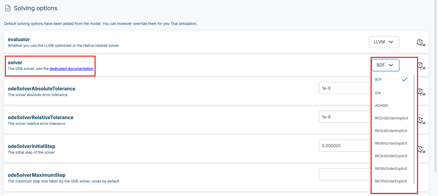
Recommended solvers

solver	Description
BDF	The Backward Differentiation Formula, Sundials CVODE's go-to method for solving stiff problems, with adaptive order ranging from 1 to 5. This is the default and recommended option.
IDA	A generalization of BDF which is able to tackle Differential Algebraic Equations (DAE). ⚠️ Note that any model including rateOf expressions or algebraic rules will automatically switch the solver to IDA.

⚠️ For advanced usage only ⚠️

The following solvers, though maintained by a trustworthy third-party library, are not as battle-tested by us as the recommended ones.

solver	Description
ADAMS	CVODE's Adams-Moulton linear multistep method, suited for non-stiff problems, with adaptive order ranging from 1 to 12.
RK2ndOrderImplicit	ARKODE's default 2nd order implicit method
RK3rdOrderImplicit	ARKODE's default 3rd order implicit method
RK4thOrderImplicit	ARKODE's default 4th order implicit method
RK3rdOrderExplicit	ARKODE's default 3rd order explicit method
RK5thOrderExplicit	ARKODE's default 5th order explicit method
RK7thOrderExplicit	ARKODE's default 7th order explicit method
RK9thOrderExplicit	ARKODE's default 9th order explicit method

Step 4: Launch and monitor

Click on the Launch Trial simulation button (bottom left) to start the simulation. 

Once a trial launched, a Simulation progress tab appears, in which you can monitor the progression of your trial pause it if needed, follow the number of numerical failures and solving speed, and have a preview of individual patients. In the case where there are numerical failures, clicking on the icon of a virtual patient will display all related patients descriptors on the right side app panel, so you can review them. 

Two other tabs will appear once the simulation is completed: 

• Subsampling design is an advanced feature allowing to calibrate a Virtual Population by adding filters or constraints on outputs or inputs of the simulation - more detail here.
• View results allows you to create a Trial visualization for more advanced post processing and visualization features than the simple one-patient preview. This is particularly interesting when you have a VPop in your trial. More details here.